The Learning Problem: Comparison between Brain and Machine

Chapter 1: The Neuron and the Perceptron

source on the left: https://www.extremetech.com/wp-content/uploads/2016/01/connectome.jpg ; on the right: https://clusterdata.nl/wp-content/uploads/2018/01/maxresdefault-1.jpg— modified by me

This is the first chapter of a series devoted to analyze and decompose the learning problem in its very bases. In doing that I would like to stress the comparison between the biological and the artificial realm. Particularly, as a Physicist, I’m interested in understanding Emergence and Self-Organization phenomena, which are topics typically related to Complex Systems (e.g. the Brain or a Deep Neural Network). The central idea will thus be: showing how well-understood solutions (e.g. a single neuron) can be applied in a bottom-up manner in order to understand complex situations. With the purpose of building a solid structure for tackling this problem we’d need two tools: Mathematical Modeling and Simulation (a.k.a. Coding). I’ll go trough all of this since the very beginning, let’s get it started!

If you can’t solve a problem, then there is an easier problem you can solve: find it. (George Pólya, Mathematical Discovery on Understanding, Learning, and Teaching Problem Solving)

Physics has been traditionally faithful to this idea: complex situations are preferentially studied on top of simple solutions. Even on the more abstract level, where issues pertaining to the general nature of constraints on cognitive processes are discussed, a physicist is likely to feel that natural language, for example, is much too complicated a subject-matter for a starting point. He is likely to try to construct a structure of increasing complexity consisting of definite realizations of simple processes possessing cognitive flavor. One of the main criteria for the selection of these stages is their analizability. Their properties can be studied in a non-abstract manner, avoiding mysterious conclusions which are brought by the blurriness of complexity.

In this way, in order to understand the learning problem, we should deal with its basic units. In particular we’re going to compare neurons and perceptrons. Let’s go on with the first one.

Neurons: biological candidates for understanding complexity [1]

A short description of the biological background is called for, even though it wouldn’t be possible, for a long time to come, to overcome Eric Kandel’s description of the neural sciences (you can check, therefore, this outstanding text for a general overview of the field). Only those features which are essential for the construction of the model will be summarized here.

The basic elements are, naturally, neurons and synapses. There is a fairly large variety of types of neurons in the human nervous system — variations are found in size, in structure and in function. As a choice of context, for the present purposes, we will consider a “canonical” type of neuron. If the underlying principles depend on the structure of individual neurons, it is unlikely that physics will contribute much to their clarification. Beyond a certain level, complex functions must be a result of the interaction of large numbers of simple elements.

Fig.1A source: https://www.forbes.com/sites/andreamorris/2018/08/27/scientists-discover-a-new-type-of-brain-cell-in-humans/ — modified by myself

Fig.1B source : https://ib.bioninja.com.au/standard-level/topic-6-human-physiology/65-neurons-and-synapses/neurons.html

A neuron is depicted in Figure1, alongside its schematic representation. The neurons communicate via synapses, which are the points along the axon of the pre-synaptic *neuron at which it can communicate the outcome of the computation that has been performed in its *soma to the dendrites or even directly to the soma of the post-synaptic neuron. The output part is the axon. Usually only one axon leaves the soma and then, downstream, it branches repeatedly, to communicate with many post-synaptic neurons.

Now, from our perspective, the dynamics of neurons and synapses, which is very similar to the propagation of an electric signal in a cable, is based on the following sequence:

• The neural axon is in an all-or-none state. In the first state it propagates a signal — spike, or *action potential — *based on the result of the summation, performed in the soma, of signals coming from dendrites. The shape and amplitude of the propagating signal is very stable and is replicated at branching points in the axon. Furthermore, the presence of a traveling impulse in the axon blocks the possibility of a second impulse transmission.

• When the traveling signal reaches the endings of the axon it causes the secretion of neuro-transmitters — *our harbingers — *into the synapse extremity.

• The neuro-transmitters arrive, across the synapse, at the post-synaptic neuron membrane and bind to receptors, thus causing the latter to open up and allow for the penetration of ionic current.

• The post-synaptic potential (PSP) diffuses in a graded manner towards the soma where the inputs from all the pre-synaptic neurons connected to the post-synaptic one are summed. If the total sum of the PSP’s arriving within a short period surpasses a certain* threshold*, the probability for the emission of a spike becomes significant.

Following the event of the emission of a spike, the neuron needs time to recover. We are going to name this amount of time as absolute refractory period, in which the neuron cannot emit a second spike (in this way nature sets a maximal spike frequency, de facto limiting the amount of information that a neuron can process in a fixed amount of time).

The previous description indicates that the only way neurons can communicate the outcome of their computations to other neurons is trough the emission of neurotransmitters. For the sake of mathematical modeling we shall make a strong assumption, namely that: sub-treshold potentials do not lead to the release of neurotransmitters. In other words, neurotransmitters are released by spikes only.

Now that we have a basic introduction of neurons functionalities we can take a look at a mathematical model, i.e. the Leaky Integrate-and-Fire (LIF) neuron. For the ones of you who are interested in the “heavy” math behind this model, I’m going to briefly introduce it.

Leaky Integrate-and-Fire model, a mathematical perspective [2]

The canonical way in order to deal with neuronal models is the circuit analogy. This is pretty technical, but I’ll try to keep it as low level as possible. For the ones of you who have taken an Electronics 101 it’ll just be a quick recap of a simple 𝑅𝐶 circuit.

We’ve been previously talking about the summation (sometimes referred as integration) process that happens in the soma, which is, combined with the mechanism that triggers action potentials above some critical threshold, the very core of neuronal dynamics.

Let’s now dive into math so that to build a phenomenological model of neuronal dynamics. We describe the critical voltage as a formal threshold 𝜽. If the voltage 𝑢(𝑡) (the sum of all inputs) reaches 𝜽 from below, we say that the neuron fires a spike. In this model we have two different components that are both necessary to define the dynamics: first, an equation that describes the evolution of the potential 𝑢(𝑡); and second, a mechanism to generate spikes.

The following is the simplest model in the class of integrate-and-fire models is made up of two ingredients: a linear differential equation to describe the evolution of 𝑢(𝑡) and a threshold for spike firing.

The variable 𝑢(𝑡) describes the instant value of the potential of our neuron. In the absence of any input, the potential is at its resting state 𝑣 . If the neuron receives an input (a current) 𝐼(𝑡), the potential 𝑢(𝑡) will be deflected from its resting value.

In order to arrive at an equation that links the momentary voltage 𝑢(𝑡) — 𝑣 to the input current 𝐼(𝑡), we use elementary laws from the theory of electricity. If a current pulse 𝐼(𝑡) is injected into the neuron, the additional electrical charge will charge the cell membrane. The cell membrane will therefore act as a capacitor of capacity 𝐶. The charge will slowly leak through the cell membrane since this ladder is not a perfect insulator. We can take this into account by adding a finite leak resistance 𝑅 to our model.

The basic electrical circuit representing a leaky integrate-and-fire model consists of a capacitor 𝐶 in parallel with a resistor 𝑅 driven by a current 𝐼(𝑡); see Figure 2

Figure2 — source : https://neuronaldynamics.epfl.ch/online/Ch1.S3.html . On the left: a neuron, which is enclosed by the cell membrane (big circle), receives a (positive) input current 𝐼(𝑡) which increases the electrical charge inside the cell. The corresponding circuit is depicted at the bottom. On the right: the cell membrane reaction to a step current (top) with a smooth voltage signal (bottom)

With the purpose of analyzing the circuit, we use the law of current conservation and split the current into two components:

The first component is the current which passes through the linear resistor 𝑅 and it can be calculated from Ohm’s law. The second component charges the capacitor 𝐶. Thus, by using Ohm’s law and the current-voltage relation for capacitors, we get:

Luckily, this is a linear differential equation in 𝑢(𝑡) and it is easy to solve, especially if we consider a constant input current 𝐼(𝑡) = 𝑖 which starts at 𝑡 = 0 and ends at time 𝑡 = 𝚫. For the sake of simplicity we assume that the membrane potential at time 𝑡 = 0 is at its resting value 𝑢(0) = 𝑣.

The solution for 0<𝑡<𝚫 is, thus:

If the input current never stopped, the potential would approach for 𝑡→ ∞ to the asymptotic value 𝑢(∞)=𝑣 +𝑅𝑖. We can understand this result by taking a look at Figure2 right-side bottom. Once a plateau is reached, the charge on the capacitor no longer changes. All input current must then flow through the resistor. Additionally, for notation purposes we usually denote RC as 𝜏, phisically the time constant of our circuit. Now that we have introduced our ingredients it’s time to start baking some code.

Let’s code a Leaky Integrate-and-Fire neuron

We’re going to use Brian2, a very efficient Python library for simulating spiking neural networks (i.e. biological neural networks), which you can easily install by following the official instructions.

I often use Jupyter notebooks in order to run Python scripts: it’s an interactive environment that let you code and integrate *Markdown *and a wide range of useful plugins specifically designed for scientific computing and machine learning.

Once you’re ready with the installation, you can start by importing Brian2.

import brian2 as br2

After that, we’re going to define some global parameters of our model: N is the number of neurons; tau is the circuit time constant, previosly defined ( i.e. 𝜏 = RC ); v_r is the resting membrane potential (i.e. 𝑣); I_c is the constant input current (i.e. 𝑖); v_th is the spike critical voltage (i.e. threshold 𝜗)

N = 1

tau  = 10 *br2.ms
v_r = 0 *br2.mV
I_c = 18 * br2.mV

#v_th is a string, it's going to be clear in a while
v_th = "v > 15*mV"

You should note that in defining the variables we’ve set physical units as well.

Consequently, we can sketch out the dynamics: Brian2 let you write the equations that describe your model, you have to specify units as well (I know the current is apparently measured in* Volt *here — it’s a kick in the teeth, but everything is done for the sake of congruence)

eqs = '''
dv/dt = -(v-I)/tau : volt
I : volt
'''

By calling NeuronGroup we’re creating a group of Neurons (here we have 1 neuron) with the previously defined dynamics, v_r and I_c as the characteristics of our neuron. In order to record its activity we call StateMonitor, v_trace can be used to extract time and voltage values as we’ll soon see.

lif = br2.NeuronGroup(N, model = eqs, threshold =v_th, reset = 'v = 0*mV')
lif.v = v_r   
lif.I = I_c

v_trace = br2.StateMonitor(lif, 'v', record = True)

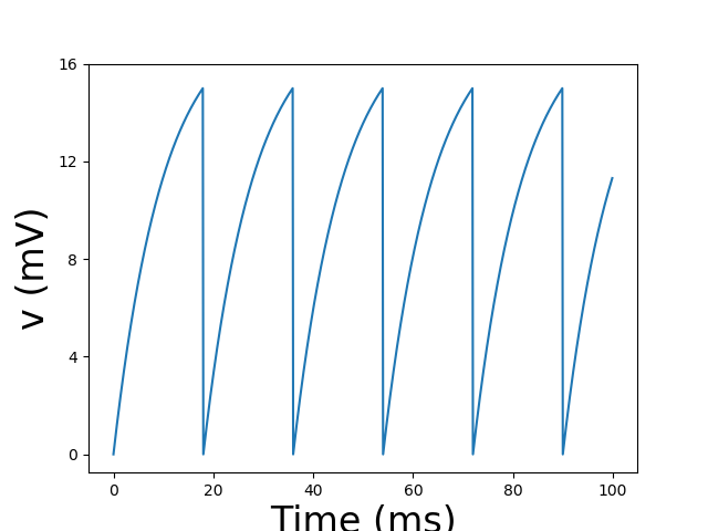
The last step consists in running the simulation and plotting the result. As previously said, we extract time from v_trace as our x-axis and voltage (*v[0] *refers to the first — and only — neuron). You have to be careful with physical units — again — and remember that for plotting we need a dimensional data.

br2.run(0.1*br2.second)

br2.figure(1)
br2.plot(v_trace.t[:]/br2.ms, v_trace.v[0]/br2.mV)
br2.xlabel('Time (ms)', fontsize = 24)
br2.ylabel('v (mV)', fontsize = 24)
br2.yticks([0,4,8,12,16])
 
br2.show()

The result is thus a sequence of spikes. You should play with parameters in order to see different kinds of behaviour.

We’ve described a fairly biological model of spiking neurons, but what’s the transition from this realm to the artificial one? Let’s talk about perceptrons.

Perceptrons: artificial candidates for understanding complexity [3] [4]

By continuing with the complex systems’ paradigm, from Minsky’s and Papert’s book:

Although we do not have an equally elaborated theory of ‘learning’, we can at least demonstrate that in cases where ‘learning’ or ‘adaption’ or ‘self-organization’ does occur, its occurrence can be thoroughly elucidated and carries no suggestion of mysterious little-understood principles of complex systems. Whether there are such principles we cannot know. But the perceptron provides no evidence; and our success in analyzing it adds another piece of circumstantial evidence for the thesis that cybernetic processes that work can be understood, and those that cannot be understood are suspect.

As hinted by the quotation above and strongly advocated by Turing, mental phenomena are nothing but an expression of a very complex structure operating on relatively simple processes. This is the very first thought that brought to the formalization of the brain.

The perceptron is, in this way, the very first brick of Artificial Intelligence. We are going to formalize the biological neuron, de facto getting the perceptron and after that introduce Rosenblatt’s perceptron learning algorithm.

We now focus on the logical structure of a single neuron. The description of the previous sections suggests the following scheme:

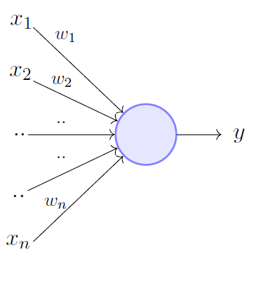Figure 3

• There is a processing unit, the large circle , which represents the soma.

• A number of input lines connect, logically, to the soma, depicted with incoming arrows in Figure3. They represent dendrites and synapses.

• The input channels are activated by the signals they receive from the input variables (x’s) to which they are connected. These variables are our pre-synaptic axons, and they have an intrinsic logical nature, since they can either activate the channel (carry a spike) or not activate it (sub-treshold activity in the pre-synaptic neuron).

To each input line, we associate a parameter* w* — the subscript refers to the various input channels. The numerical value of each w is indeed the amount of post-synaptic potential (PSP) that would be added to the soma if the channel were activated.

Furthermore, there is a single logical output line (outgoing arrow in Fig3). It expresses the logical fact that our neuron produces a single relevant ouput — a spike .

We can arrange the operations of the unit in the following way:

• At a given moment, some of the logical inputs are activated.

• The soma receives an input which is the linear sum of PSP values of the channels that were activated — the variable x indicates whether the channel is active (x = 1) or inactive (x = -1)

• The sum of PSP’s is compared to the threshold value of the neuron and the output channel is activated if it overcomes the threshold.

Formally, we’ll get:

with h as the PSP at our neuron and n as the number of pre-synaptic neurons. Mathematically h is nothing but a dot product.

Anyways, the operation implemented by our little “machine” can be expressed as:

with sign as the sign function and 𝜽 as the threshold of our neuron. H is basically 1 if its argument (h+𝜽) is positive and -1 if negative — and, to be precise, 0 if h +𝜽 = 0. The variable y indicates, in our biological analogy, whether a spike will appear in the output axon.

Now that our perceptron has taken shape we can talk about how this mathematical structure can be involved in the learning process. Let’s introduce Rosenblatt’s perceptron learning algorithm.

The learning process in perceptrons [4]

There’s a clear analogy between neurons and perceptrons, but how can we use this ladder model in order to learn ? We’re going to show that the perceptron can be used to solve classification problems, namely it can tell you whether, if we have two sets of points, a point belong to one set or another. We can say without a lack of generalizability that the problem can be thought as a binary (yes/no) decision, where the variable y (the output value) defined above is one of these two binary values ( yes = 1, no = -1) .

From the previous definition of h as a dot product it’s even clearer that x is formally a vector (the input vector). Every component of x is called feature, by talking in Machine Learning terms. In the same way w is a vector (the weight vector). The threshold term 𝜽 it’s usually called bias term. In the direction of a simplified notation we’re going to augment both x and w in the following way:

Basically, by extending the sum from i = 0 to i = n.

The learning algorithm we’re going to build will consider all these terms and in particular the term learning specifically refers on finding the best value of w’s components in order to achieve the best classification possible. Take a look at the following 2-dimensional (here x has only two components) problem in Figure4 and everything will be clear.

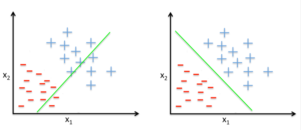Figure 4 — On the left: misclassified data. On the right: perfectly classified data.

So, in practice, classification means finding a way in order to separate the two different “kinds” of data we have. Each “kind” of data is specified by a different label (plus or minus, in the figure above). So to speak, this is a two labels classification problem.

It’s time to introduce the perceptron learning algorithm (PLA), which will determine what w should be, based on the data. This learning algorithm consists in a simple iterative method. By involving the term “iteration”, we’re going to introduce a new parameter in our model, namely, time. At iteration t, where t = 0,1,2…, there is a current value of the weight vector, call it w(t). The algorithm picks a point, associated with its label, that is currently misclassified, call it (x(t), y(t)), and uses it to update w(t). Since the example is misclassified, we have *y(t) ≠ sign(w(t) · x(t)), where the dot represents the dot product.

The weight update rule is as follow:

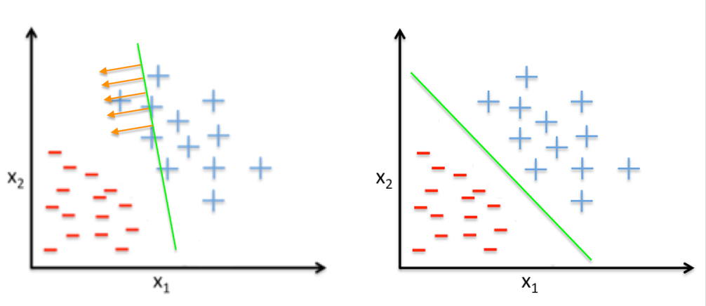Figure 5 — The last update

This rule moves the boundary in the direction to classify x(t) correctly, as depicted in the figure above. The algorithm continues with further iterations until there are no longer misclassified points in the data set. With this intuitive view of the PLA, it’s now time to code it.

Let’s code the Perceptron Learning Algorithm

We’re going to implement the PLA from scratch by coding a simple Python script. Let’s open a new notebook with Jupyter and start by importing matplotlib.pyplot and numpy

import matplotlib.pyplot as plt
import numpy as np

We’re going to create a 2-dimensional random dataset of 5 points (with two possible labels, -1 and +1) by using numpy.random.rand(). In order to reproduce the result we’ll fix the random seed — you can actually choose every integer number, 137 has a particular meaning for Physicists though.

# Setting the random seed 
np.random.seed(seed = 137)

# Generate x1 and x2, coordinates of our points
number_of_points = 5
x1 = np.random.rand(number_of_points)
x2 = np.random.rand(number_of_points)

# We have two labels, namely -1 and 1
possible_ys = np.array([-1,1])

# We randomly build the label y to point (x1,x2) association 
y = np.random.choice(possible_ys, number_of_points)

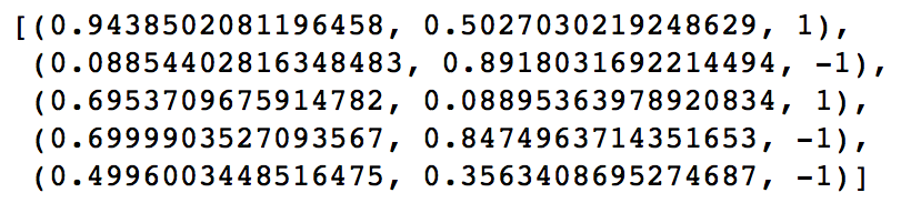
Data are represented by triplets of values.

# We create data as triplets of values
data = []
for i in range(number_of_points):
    data.append((x1[i],x2[i],y[i]))

You can take a look at your data by executing the following line and you’ll get:

# Taking a look at data
data

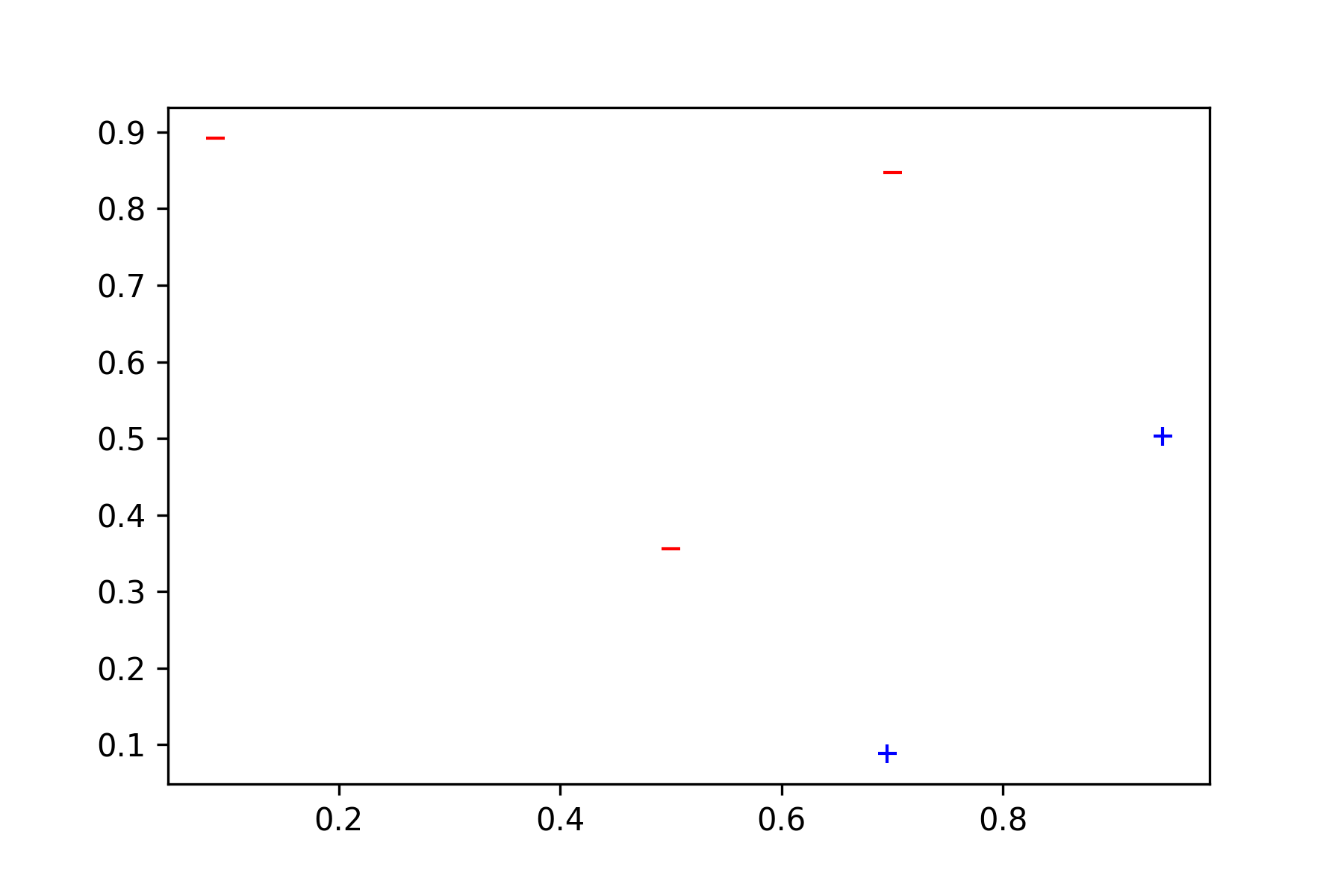
The next step is to plot them by denoting with a “-” the label corresponding to “-1” and by “+” the label corresponding to “1”

# Plotting our data 
plt.plot([x1 for (x1,x2,y) in data if y==-1], [x2 for (x1,x2,y) in data if y==-1], '_', mec='r', mfc='none')
plt.plot([x1 for (x1,x2,y) in data if y==1], [x2 for (x1,x2,y) in data if y==1], '+', mec='b', mfc='none')

After that we can start with the learning model. The very first thing to do is to initialize the weights, usually a “little” random value is the best solution for faster convergence.

# Initializing the weight vector
w = np.random.rand(3)*10e-03

Consequently, we define the function “predict” which is nothing but sign(w(t) · x(t))

def predict(x1,x2):
    # w[0] is the threshold value, x0 = 1 
    h= w[0] + w[1]*x1 + w[2]*x2
    
    if h<0:
        return -1
    else:
        return 1

The last part of the learning model is the function “fit” which corresponds to the weight update rule. The essence is: for every point we compare the predicted label with the actual one, if these are not equal each component of the weight vector is updated.

def fit(data):
    stop = False
    
    while stop == False:
        stop = True
        
        for x1,x2,y in data:        
            ypredict= predict(x1,x2) 
            if y != ypredict: 
                              
                stop = False
            
                w[1]= w[1] + x1*y
                w[2]= w[2] + x2*y
                w[0]= w[0] + y

By applying the function “fit” to our data, the PLA will converge to a solution. If this is the case we’ll get a printed ‘SUCCESS!’ as the output of the following cell.

fit(data)

# Check if the model is predicting correct labels
for (x1, x2, y) in data:
    if predict(x1,x2) != y:
        print('FAIL')
        break
else:
    print('SUCCESS!')

Last but not least, we can plot our result. “f(x)” is the functional form of the line given by the PLA(you can get it by applying simple algebraic calculations — de facto by expliciting the expression for x2).

def f(x):
    return -(w[0] + w[1]*x)/w[2]

d = range(0,2)
plt.plot(d, [f(x) for x in d])

plt.plot([x1 for (x1,x2,y) in data if y==-1], [x2 for (x1,x2,y) in data if y==-1], '_', mec='r', mfc='none')
plt.plot([x1 for (x1,x2,y) in data if y==1], [x2 for (x1,x2,y) in data if y==1], '+', mec='b', mfc='none')

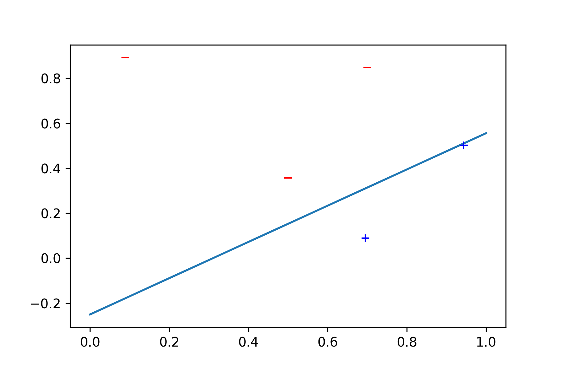
In this way, we’ve solved a simple classification problem, i.e. we’ve been learning!

Conclusions

We’ve reached the end of our adventure: we’ve been traveling trough a mathematical model of the neuron and its implementation. With that in mind,we’ve been taking inspiration from it in order to formalize the neuron and build the perceptron. Be careful though, the perceptron is not a biologically plausible model. The relationship between neurons and pereptrons is much more similar to the one between birds and planes. Here, the problem of “flying” is actually the learning problem, but again, the road for a perfectly reliable plane it’s way longer than this.

In particular perceptrons have an intrinsic problem, which is insurmountable without a major change. Minsky and Papert have been pointing out that issue so clearly that research in Artificial Intelligence has been subjected to a quite long break. Therefore, I would like you to point out this serious perceptron’s limitation. I think that you can grasp an intuition of the problem by looking at the code in the previous section and tweaking np.random.seed() and number_of_points. Give it a try and let me know!

References

[1] Amit, D. (1989). Modeling Brain Function: The World of Attractor Neural Networks. Cambridge: Cambridge University Press.

[2] Wulfram Gerstner, Werner M. Kistler, Richard Naud, and Liam Paninski. 2014. Neuronal Dynamics: From Single Neurons to Networks and Models of Cognition. Cambridge University Press, New York, NY, USA. Online version: *https://neuronaldynamics.epfl.ch/online/index.html

[3] Marvin L. Minsky and Seymour A. Papert. 1988. Perceptrons: Expanded Edition. MIT Press, Cambridge, MA, USA.

[4]Rosenblatt, Frank. 1962. Principles of neurodynamics; perceptrons and the theory of brain mechanisms. Washington, Spartan Books

[5] Yaser S. Abu-Mostafa, Malik Magdon-Ismail, and Hsuan-Tien Lin. 2012. Learning from Data. AMLBook.