A Reinforcement Learning Algorithm for Reducing Energy Consumption

Progress in urbanization and advancement of the “fully connected” society is giving electricity more and more importance as the main energy source for our social life. Electricity, like air and water, is so widespread that nobody may notice its existence. In view of the increase in its demand, the electric power system has come to face three adversely affecting issues, namely: energy security, economic growth, and environmental protection. Or else, if supply of electricity is stopped, our society will be thrown into a terrible chaos.

The need of energy savings has become increasingly fundamental in recent years. Especially, with regards to energy consumption due to buildings we are around the 40% of the global energy [1]. The most effective way to reduce energy consumption of existing buildings is retrofitting(i.e. the addition of new technology or features to older systems), and one of its implementations pass trough efficient Heating, Ventilation and Air Conditioning (HVAC) systems.

Traditionally HVAC systems are controlled by model-based (e.g. Model Predictive Control) and rule-based controls.

In the last decade a new class of controls which relies on Machine Learning algorithms have been proposed. In particular, we are going to highlight data driven models based on Reinforcement Learning (RL), since they showed from the very beginning promising results as HVAC controls [2]. But first, let us dig deeper in these control methods.

Model Predictive Control (MPC)

The basic MPC concept can be summarized as follows. Suppose that we wish to control a multiple-input, multiple-output process while satisfying inequality constraints on the input and output variables. If a reasonably accurate dynamic model of the process is available, model and current measurements can be used to predict future values of the outputs. Then the appropriate changes in the input variables can be calculated based on both predictions and measurements. Thus, the changes in the individual input variables are coordinated after considering the input-output relationships represented by the process model.

In essence MPC can fit to complex thermodynamics and achieve good results in terms of energy savings on a single building. Following this train of thought, there is a major issue: the retrofit application of this kind of models requires to develop a thermo-energetic model for each existing building. Similarly, is clear that the performance of the model relies on its own quality and having a pretty accurate model is usually expensive. High initial investments are one of the main problems of model-based approaches [3]. In the same fashion, for any intervention of energy efficiency on the building, the model has to be rebuilt or tuned, again, with an expensive involvement of a domain expert.

Rule-Based Controls (RBC)

Rule-based modeling is an approach that uses a set of rules that indirectly specifies a mathematical model. This methodology is especially effective whenever the rule-set is significantly simpler than the model it implies, in a way such that the model is a repeated manifestation of a limited number of patterns.

RBC are, thus, state-of-the-art model-free controls that represents an industry standard. A model-free solution can potentially scale up, because the absence of a model makes the solution easily applicable on different buildings without the need for a domain expert. The main drawback of RBC is that they are difficult to be optimally tuned because they are not enough adaptable with respect to the intrinsic complexity of the coupled building and plant thermodynamics.

Reinforcement Learning Controls

Before introducing the advantages of Reinforcement Learning Controls we are going to talk briefly about Reinforcement Learning itself. Using the words of Sutton and Barto [4]:

Reinforcement learning is learning what to do — how to map situations to actions — so as to maximize a numerical reward signal. The learner is not told which actions to take, but instead must discover which actions yield the most reward by trying them. In the most interesting and challenging cases, actions may affect not only the immediate reward but also the next situation and, through that, all subsequent rewards. These two characteristics — trial-and-error search and delayed reward — are the two most important distinguishing features of reinforcement learning.

In our case, a RL algorithm interacts directly with the HVAC control system and adapts continuously to the controlled environment using real-time data collected on site, without the need to access to a thermo-energetic model of the building. In this way a RL solution could obtain primary energy savings reducing the operating costs while remaining suitable to a large-scale application.

Therefore, it is very attractive to introduce RL controls for large-scale applications on HVAC systems where the operating cost is high, like those in charge of the thermo-regulation of a great volume.

One of the building use classes where it could be convenient to implement a RL solution is the supermarket class. Supermarkets are, by definition, widespread buildings with variable thermal loads and complex occupational patterns that introduce a non-negligible stochastic component from the HVAC control point of view.

We are going to formalize this problem by using the framework of Reinforcement Learning, let us contextualize it in a better way.

A Reinforcement Learning Solution

In RL an agent interacts with an environment and learns the optimal sequence of actions, represented by a policy to reach a desired goal. As reported in [4]:

The learner and decision maker is called the agent. The thing it interacts with, comprising everything outside the agent, is called the environment. These interact continually, the agent selecting actions and the environment responding to these actions and presenting new situations to the agent.

Figure 1 : ResearchGate

In our work, the environment is a supermarket building. The learning goal of the agent is expressed by a reward: a scalar value returned to the agent which tells us how the agent is behaving with respect to the learning objective.

The interaction between agent and environment leads to a decision process: the reward acts as a feedback. We formalize this interaction by means of a Markov Decision Process (MDP) which is completely described by means of a finite ordered list — i.e. a tuple — ( S, A, r, 𝑃 ), where S is the set of states, A is the set of actions, r: SｘA→ R is the reward function and 𝑃 is the transition probability from a state-action pair to the next state 𝑃 : Sｘ Aｘ S→ [0,1].

Intuitively speaking, we can decide how to solve a decision-making problem whenever we know where we are (S), which actions we can take (A), whether the previous action is good or not (r) and where the next action is more likely to take us (𝑃 ). The term Markov is, in fact, related to the Markovian assumption, i.e. the state observed by the agent completely represents the useful information about the environment. In real applications we have that the Markovian assumption is relaxed in favor of a “quasi-Markovian” condition, the agent cannot observe the complete representation of the environment: “the state observed by the agent approximates the actual state” [4].

During a sequence of time-steps (time is discrete), the agent improves its policy π : S→ ℙ(A), which represents its behavior in the environment, where ℙ(A) is a probability distribution over the set of actions. The goal of the policy improvement procedure is to get to the optimal policy π, defined as the policy that maximizes the expected discounted return:

where 𝛾 ∈ [0,1]

Again, informally, the policy is nothing but the “dynamical” strategy that our agent is engaging to do.

Translating this formalism to HVAC control systems, the goal of the RL algorithm is to save energy while satisfying comfort constraints. In this kind of problem we usually have to take into account a trade-off between comfort components and primary energy consumed.

The comfort constraint is defined as an acceptable interval of the internal air temperature [T¹, T²], where T¹ and T² both depend on the season. For instance, the interval [T¹, T²] is fixed to [16°C, 19°C] for the winter season and [23°C, 25°C] for summer [5].

Consequently, the reward at each time-step as the sum of two components, the first is related to the cost and the second to the comfort:

The two components are defined as:

Where c is the sum of electric and thermal energy costs, updated at each time-step, λ is a trade-off parameter between the comfort and the cost component and p is the constraint penalization factor defined as:

The exponential function applied to p accounts for the greater importance of the comfort component as the temperature is out of the comfort range.

In real applications we need to find a way to estimate the comfort level in the controlled zone, in order to tune the parameter λ. Mathematically we can solve this by thinking about the comfort constraint (i.e. that T is in the interval [T¹, T²]) as a stochastic constraint. The idea is that given a temperature T and a possible exceeding value 𝛥T, the agent can let the temperature exceed T+𝛥T only with a bounded probability.

Technically speaking, to define the stochastic constraint, we first compute the empirical probability density function of the internal air temperature values T registered for each hour of the day. We can see an example of such densities for different control systems in Figure 2.

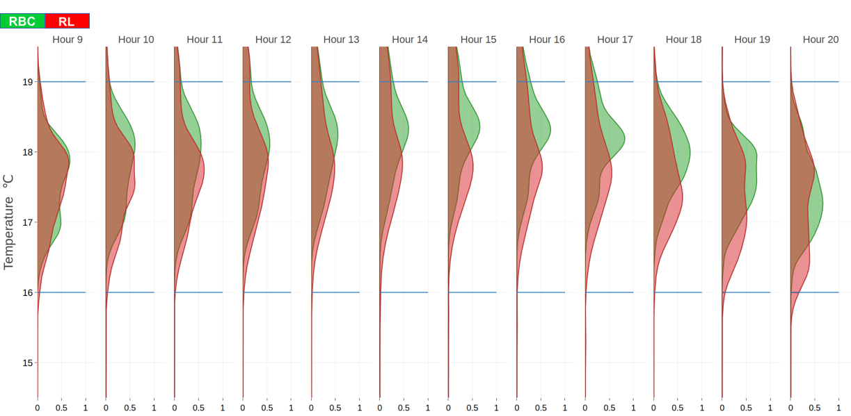Figure 2: Example of the temperature reached by the RL method (red) and the RBC method (green) in a working day of the winter testing period. The areas show the empirical pdf of the temperature, during the opening time, grouped by hour.

The RL algorithm, as previously introduced, improves continuously its policy by collecting information about the environment dynamics. In order to complete our recipe, we need one more ingredient: the q-function. The expected value of the return obtained by starting in a state s, choosing an action a and following a policy π is called q-function for the policy π:

Our agent is going to compute an approximation of q (i.e. Q or Q-function) for every pair (s,a).

The optimal policy satisfies the Bellman optimality equation:

Which opens a lot of doors for iterative approaches in order to get to an optimal Q-function. This, in fact, leads to the Q-learning algorithm: after a transition (i.e. a time-step), the Q-function is updated in the following way:

where 𝛼 ∈ [0,1] is the learning rate. To improve the Q-function approximation is even possible to extend this formalism to K consecutive transitions, namely, we are going to memorize multiple time-steps and introduce them in the evaluation of the Q-function in order to get a more precise value.

When the state and action spaces are finite and small enough, the Q-function can be represented in tabular form, and its approximation as well as the control policy derivation are straightforward. However, when dealing with continuous or very large discrete state and action spaces, the Q-function cannot be represented anymore by a table with one entry for each state-action pair.

In practice, the application of RL to HVAC control suffers from the curse of dimensionality: it needs a non-linear regression algorithm because of the high dimensionality of the state space together with the non-linearity of the building dynamics.

To overcome this generalization problem a particularly attractive framework is the one used by Ernst [6] which applies the idea of fitted value iteration (i.e. Fitted Q-Iteration or FQI), where the regression is computed by means of an* Extremely Randomized Tree *[7].

FQI belongs to the family of batch-mode RL algorithms. The term “batch-mode” refers to the fact that the algorithm is allowed to use a set of transitions of arbitrary size to produce its control policy in a single step. Basically, FQI assumes that a buffer (i.e. a set) of past transitions:

has been collected, where* t* is the current time-step.

Then it iterates the regression to the set of transitions in order to improve the accuracy of the Q-function approximation Q̂. The algorithm returns a response variable value for each transition, by using Multi-Step Q-Learning:

The Q̂ approximator at the Nth-step is used to derive a new policy and, thus, acquire new transitions. For the sake of completeness we summarize the pseudo-code of this algorithm, named as Multi-Step Fitted Q-Iteration (MS-FQI) in Figure 3

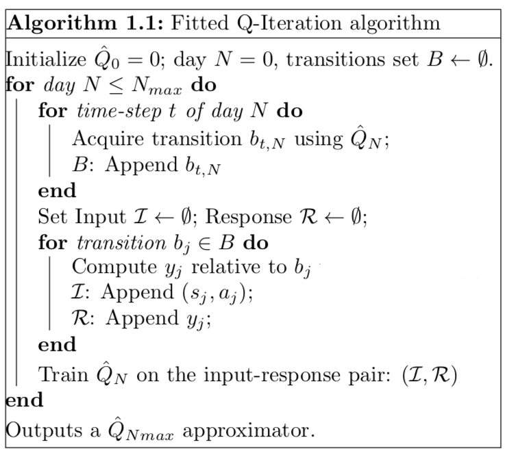Figure 3: Fitted Q-Iteration algorithm pseudo-code.

For a further improvement, we coupled this algorithm with an ε-greedy policy in order to explore the environment and not to get stucked in local minima.

What is an ε-greedy policy?

Greedy action selection always exploits current knowledge to maximize immediate reward; it spends no time at all sampling apparently inferior actions to see if they might really be better. A simple alternative is to behave greedily most of the time, but every once in a while, say with small probability ε, instead select randomly from among all the actions with equal probability, independently of the action-value estimates. We call methods using this near-greedy action selection rule ε-greedy methods.

In our case, the policy requires the agent to choose with probability 1-ε the action with the maximum estimated Q-value and with probability ε a random action.

Conclusions

By using the previously introduced RL framework, [EnergyPlus 8.5](https://energyplus.net/). in order to develop the building model and [B**uilding **C**ontrols **V**irtual **T**est **B**ed 1.5.0](https://simulationresearch.lbl.gov/projects/building-controls-virtual-test-bed). (BCVTB**) for the communication interface, we define the complete simulation framework.

Our approach shows that a RL control is a viable solution for retrofitting, especially where design values are not sufficient anymore to guarantee thermal comfort requirements because of degradation of the HVAC system. As RL control learns by interaction with environment, it can achieve savings in every climate zone. To maximize energy savings and obtain near optimal control, a re-tuning of the *λ **trade-off parameter should be taken into consideration when changing climate zone. A peculiar improvement consists in the training period of *12 months which leads to a consistent reduction with respect to the current state-of-the-art.

References

[1] Prez-Lombard, L., J. Ortiz, and C. Pout (2008, 01). A review on buildings energy consumption information. Energy and Buildings 40, 394–398.

[2] *Ruelens, F., S. Iacovella, B. Claessens, and R. Belmans *(2015). Learning agent for a heat-pump thermostat with a set-back strategy using model-free Reinforcement Learning. Energies 8 (8), 8300– 8318.

[3] Sturzenegger, D., D. Gyalistras, M. Morari, and R. S. Smith (2016). Model predictive climate control of a Swiss office building: implementation, results, and cost–benefit analysis. IEEE Transactions on Control Systems Technology 24(1), 1–12.

[4] Sutton, R. S. and A. G. Barto (1998). Introduction to Reinforcement Learning, Volume 135. MIT press Cambridge.

[5] Stefanutti, L. (2001). Impianti di climatizzazione. Tipologie applicative [HVAC Systems. Applications]. Tecniche nuove.

[6] Ernst, D., P. Geurts, and L. Wehenkel (2005). Tree-based batch mode Reinforcement Learning. Journal of Machine Learning Research 6, 503–556.

[7] Geurts, P., D. Ernst, and L. Wehenkel (2006). Extremely randomized trees. Machine Learning 63(1), 3–42.